python_bootcamp_team13
Team13: Capstone project of Python Bootcamp
This is the Capstone project for Team 13 of the Python Data Analysis Bootcamp. We are trying, more or less, to follow the structure of jupytemplate.
Purpose
State the purpose of the notebook.
Methology
Quickly describe assumptions and processing steps.
TODO / Improvements
- Find a dataset that has at least 2 CSV files
- Come up with 5 questions that you want to answer while exploring the dataset
- Perform EDA (Exploratoty Data Analysis) on your dataset with basic visualisations
Results
Setup
# install system dependencies
import sys
import os

!conda install -c conda-forge --yes --prefix {sys.prefix} pandas jupyterthemes seaborn jupyter_contrib_nbextensions pandoc
Collecting package metadata (current_repodata.json): done
Solving environment: done

# All requested packages already installed.
Library Import
# load libraries and setup environment
# mandatory
import pandas as pd

%matplotlib inline
import matplotlib.pyplot as plt

# optional
import numpy as np
import seaborn as sns
from jupyterthemes import jtplot
from IPython.core.display import HTML
jtplot.style(theme='monokai', context='notebook', ticks=True, grid=False)
Parameter definition
We set all relevant parameters for our notebook. By convention, parameters are uppercase, while all the other variables follow Python’s guidelines.
COAST_COLUMN = "Coastline (coast/area ratio)"
COUNTRY_COLUMN = 'Country'
SATISFACTION_COLUMN = "People with highest life satisfaction [%]"
Data import
We retrieve all the required data for the analysis.
cost_of_living = pd.read_csv('../data/andytran11996_cost-of-living/datasets_73059_162758_cost-of-living-2018.csv')

# we are droppping the Rank column because it's entirely empty
cost_of_living = cost_of_living.drop(columns = 'Rank')

life_satisfaction = pd.read_csv('../data/roshansharma_europe-datasets/datasets_231225_493692_life_satisfaction_2013.csv')
life_satisfaction = life_satisfaction.rename(columns = { "prct_life_satis_high": "People with highest life satisfaction [%]", "country": "Country" })
life_satisfaction['Country'] = life_satisfaction['Country'].astype(str)
life_satisfaction['Country'] = life_satisfaction['Country'].str.strip()

generic_country_data = pd.read_csv('../data/fernandol_countries-of-the-world/datasets_23752_30346_countries of the world.csv', decimal=',')
generic_country_data['Country'] = generic_country_data['Country'].astype(str)
generic_country_data['Country'] = generic_country_data['Country'].str.strip()
generic_european_country_data = generic_country_data[generic_country_data['Region'].str.contains('EUROPE', case = False)]

print('successfully imported the datasets.')
successfully imported the datasets.
Data processing
1. What are the five cities with the highest/lowest cost of living (incl. rent)?
caption_column = 'City'
index_column = 'Cost of Living Plus Rent Index'

def display_cost_of_living(costs, title):
    filtered_costs = costs[[caption_column, index_column]].sort_values(index_column, ascending = True)
    filtered_costs.plot.barh(title = title, x = caption_column, y = index_column)
    plt.show();
    display(filtered_costs.sort_values(index_column, ascending = False).style.hide_index())

# print the ten most expensive cities in the database in 2018
display_cost_of_living(cost_of_living.nlargest(5, index_column), 'Largest Rent Index')
display_cost_of_living(cost_of_living.nsmallest(5, index_column), 'Smallest Rent Index')
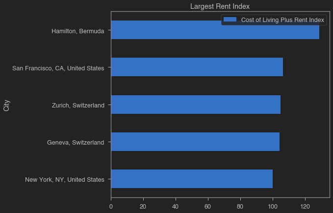
| City | Cost of Living Plus Rent Index |
|---|---|
| Hamilton, Bermuda | 128.760000 |
| San Francisco, CA, United States | 106.290000 |
| Zurich, Switzerland | 105.030000 |
| Geneva, Switzerland | 104.380000 |
| New York, NY, United States | 100.000000 |
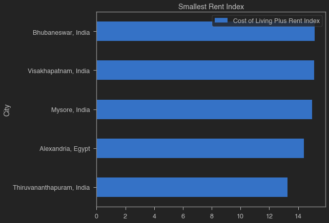
| City | Cost of Living Plus Rent Index |
|---|---|
| Bhubaneswar, India | 15.140000 |
| Visakhapatnam, India | 15.110000 |
| Mysore, India | 14.980000 |
| Alexandria, Egypt | 14.400000 |
| Thiruvananthapuram, India | 13.260000 |
2. What are the five happiest countries in Europe?
index_column = "People with highest life satisfaction [%]"
caption_column = 'Country'

top_countries_life_satisfaction = life_satisfaction[[caption_column, index_column]]
top_countries_life_satisfaction = top_countries_life_satisfaction.nlargest(5, index_column)
top_countries_life_satisfaction = top_countries_life_satisfaction.sort_values(index_column, ascending = True)
top_countries_life_satisfaction.plot.barh(title = 'Percentage of satisfied people', x = caption_column, y = index_column);
plt.show();
display(top_countries_life_satisfaction.sort_values(index_column, ascending = False).style.hide_index())
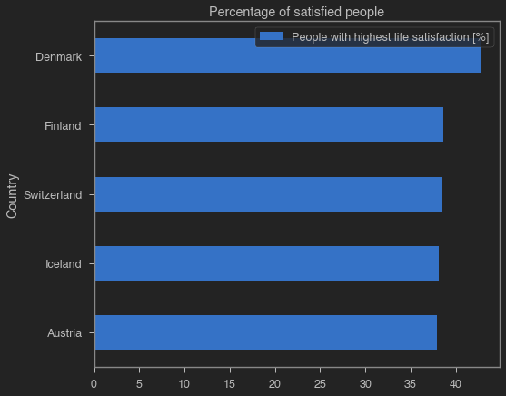
| Country | People with highest life satisfaction [%] |
|---|---|
| Denmark | 42.700000 |
| Finland | 38.600000 |
| Switzerland | 38.500000 |
| Iceland | 38.100000 |
| Austria | 37.900000 |
3. What are the European countries with the most coast line in relation to their area?
index_column = "Coastline (coast/area ratio)"
caption_column = 'Country'

coastline_data = generic_european_country_data[[caption_column, index_column]]

coastline_data = coastline_data.nlargest(5, index_column)
coastline_data = coastline_data.sort_values(index_column, ascending = True)
coastline_data.plot.barh(title = 'Countries with the most coast line in relation to their area', x = caption_column, y = index_column);
plt.show();
display(coastline_data.sort_values(index_column, ascending = False).style.hide_index())
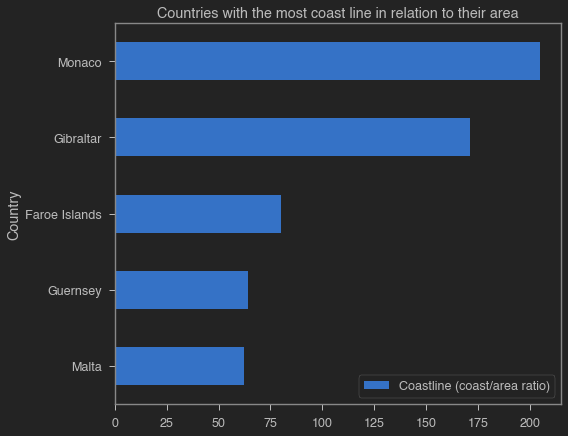
| Country | Coastline (coast/area ratio) |
|---|---|
| Monaco | 205.000000 |
| Gibraltar | 171.430000 |
| Faroe Islands | 79.840000 |
| Guernsey | 64.100000 |
| Malta | 62.280000 |
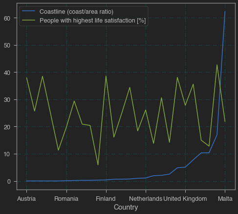
4. Is there a correlation between happiness and access to a coastline?
merged = pd.merge(generic_european_country_data, life_satisfaction, on = COUNTRY_COLUMN, how = 'inner')

coastline_data = generic_european_country_data[[COAST_COLUMN, COUNTRY_COLUMN]]

# sort by coast
merged = merged.sort_values(COAST_COLUMN, ascending = True, ignore_index = True)

ax = plt.gca()
merged.plot(kind = 'line', y = COAST_COLUMN, x = COUNTRY_COLUMN ,ax=ax)
merged.plot(kind = 'line', y = SATISFACTION_COLUMN, x = COUNTRY_COLUMN ,ax=ax)

plt.grid(b = True, color = 'aqua', alpha = 0.1, linestyle = 'dashdot')
plt.show();